
Linear equation with one variable
Function Builder by PhET Interactive Simulations, University of Colorado Boulder, licensed under CC-BY-4.0 (https://phet.colorado.edu)
Objective:
- To solve linear equations with one variable.
This virtual activity is designed to be used in math lessons in the next chapter:
- Grade 6. “Linear equation with one variable”.
Theoretical part
1. Definition:
A linear equation with one variable is an equation of the formaah+b=0, where:
a and b are arbitrary numbers (coefficients of the equation), wherea0.
x is the unknown variable.
2. Examples:
- 3x – 5 = 0
- -2x + 7 = 0
- 0.5x – 12.3 = 0
3. Solving a linear equation:
Goal: To find all values of the variable x at which the equation becomes true.
Algorithm:
- Move all terms containing x to one side of the equation.
- Move the free term (the number without x) to the other side of the equation.
- Bring similar terms in both parts of the equation.
- Divide both parts of the equation by the quotient at x.
Example:
3x – 5 = 0
3x = 5
x = 5/3
Answer: x = 5/3.
Virtual Experiment
On the equation screen, students can interpret, compare, and translate multiple representations of an algebraic function. It can predict the output of a function on given inputs and create a new function.
Workflow:
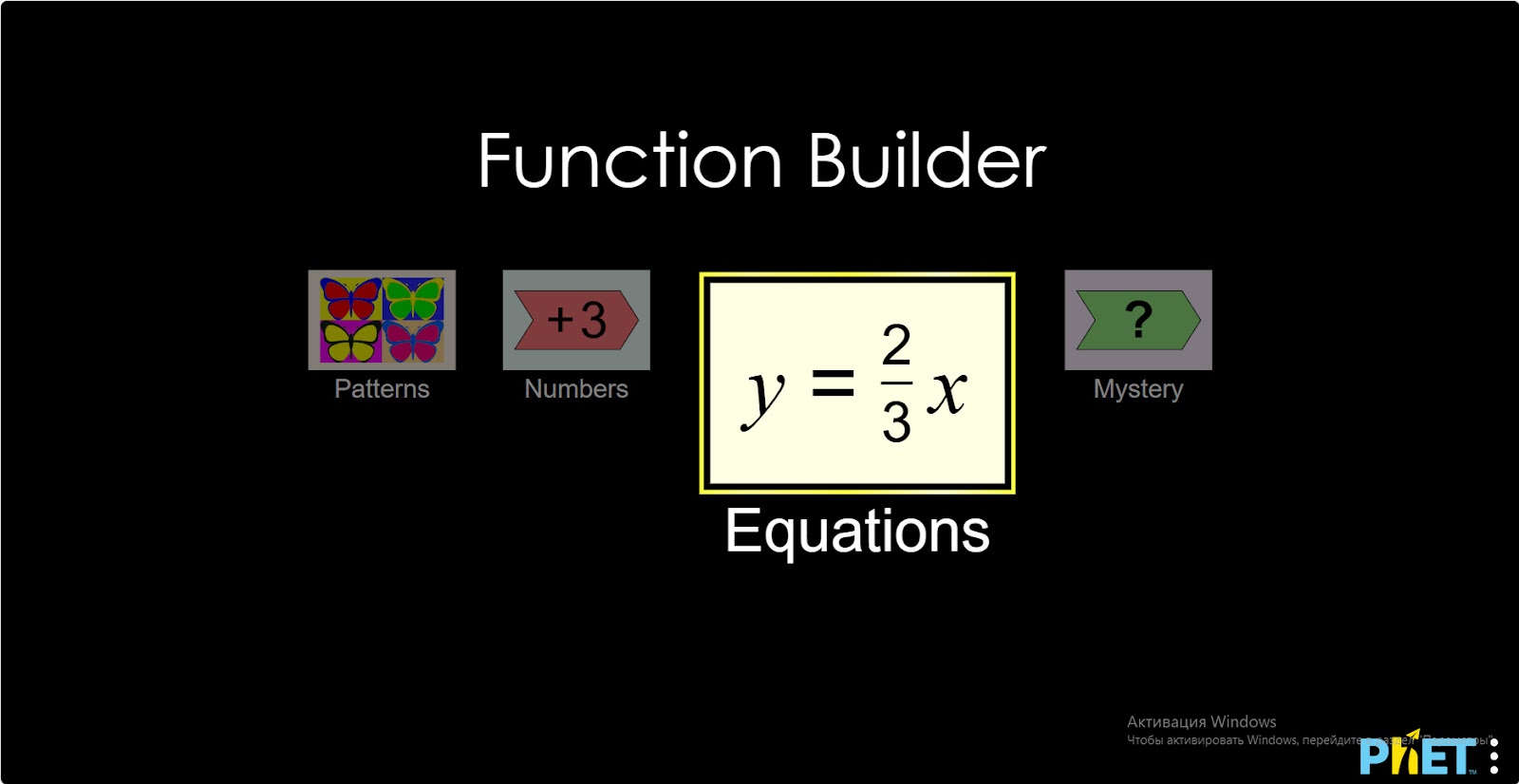
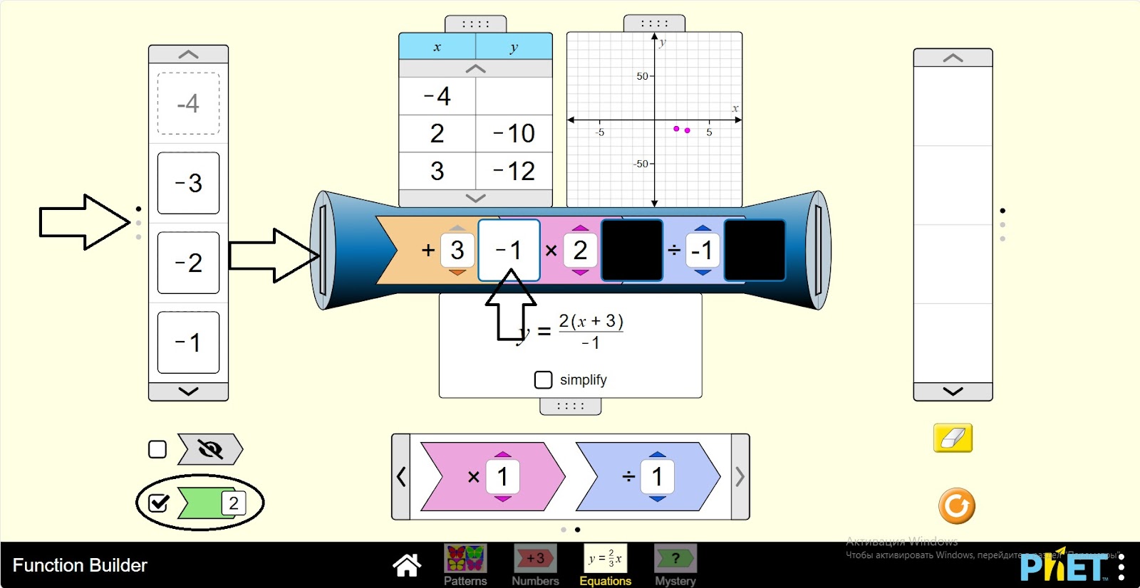
Step 1. Start the simulation: you will be presented with 4 different modes: “Patterns”, “Numbers”, “Equations” and “Mystery”. You will work on this experiment in the “Equations” section. Open the “Equations” section.
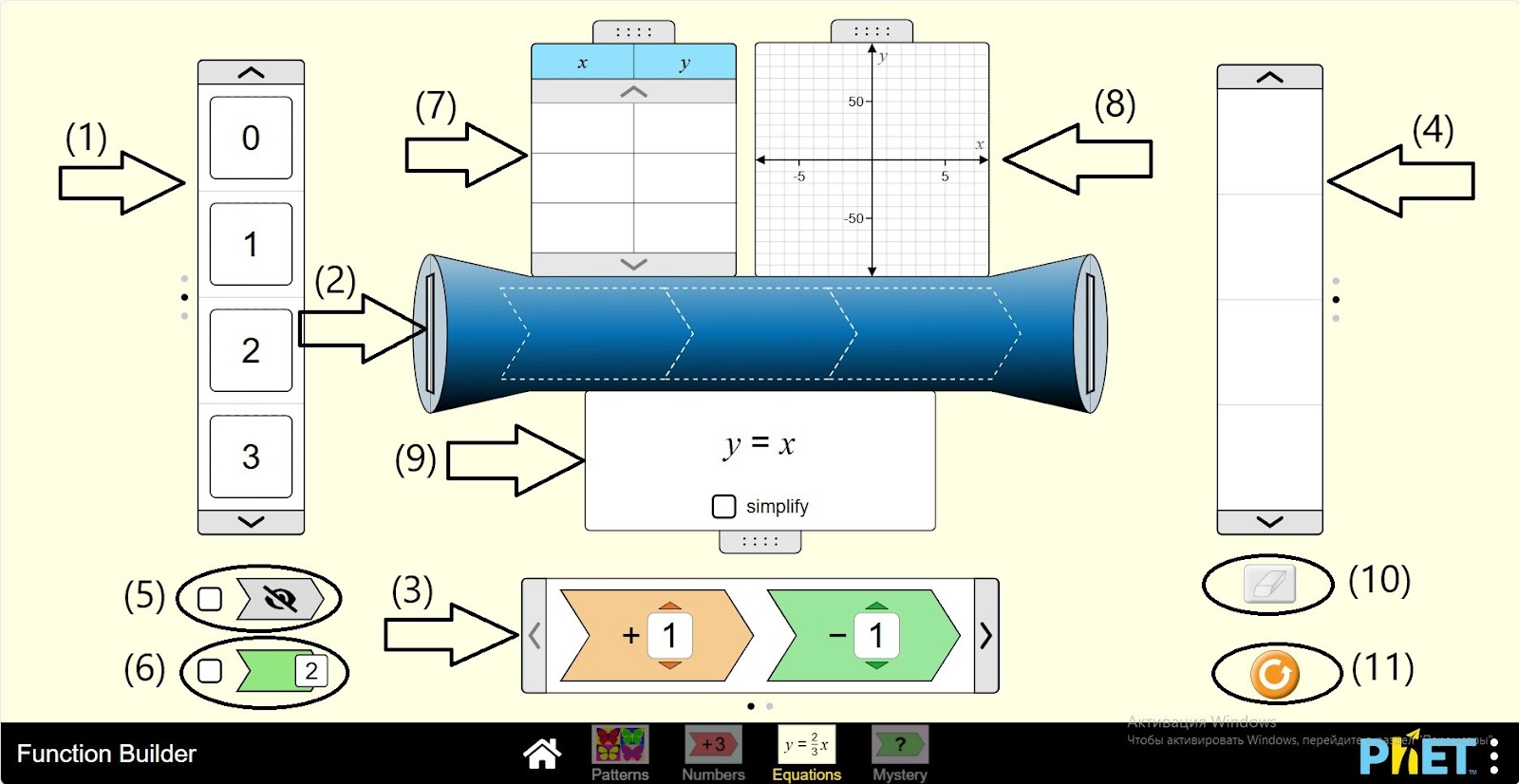
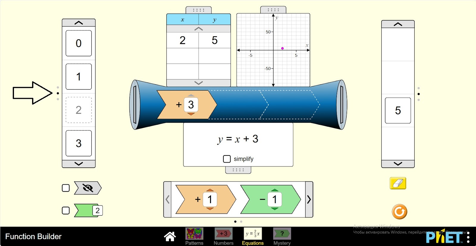
Step 2 You are given:
- Input number panel (1);
- Function machine (2);
- Arithmetic operations and numbers to construct the function (3);
- A panel of function values (4);
- Button hiding the operations located on the function machine (5);
- Button showing the value of the expression after each operation performed with the input number on the function machine (6);
- A table showing the input numbers and the value of the function on the function machine (7);
- A table showing the graph of the function on the function machine (8);
- Table showing the type of equation in the function machine (9);
- Eraser function to erase numbers in the value bar (10);
- The reset button (11).
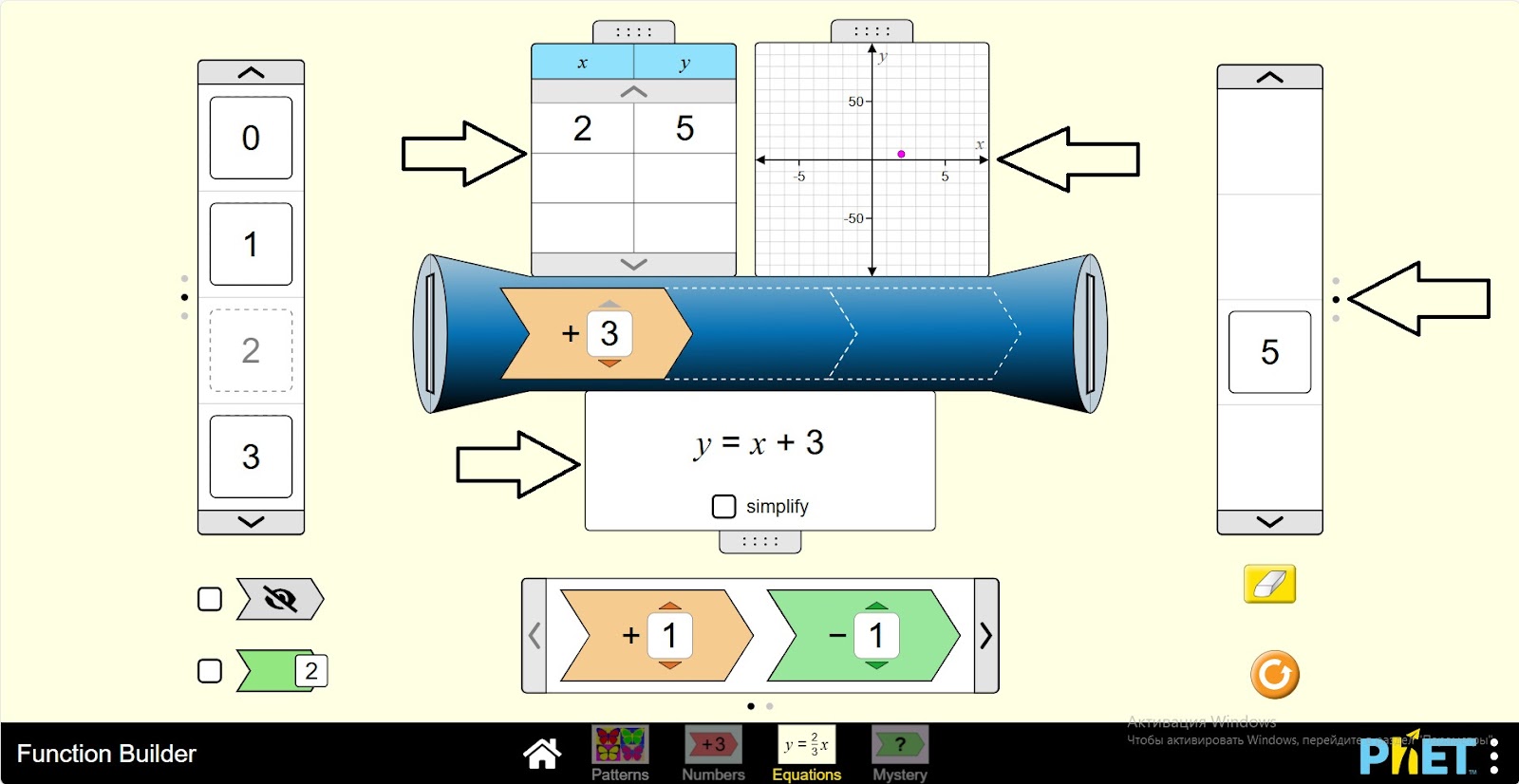
Step 3. Open the tables on the function machine.
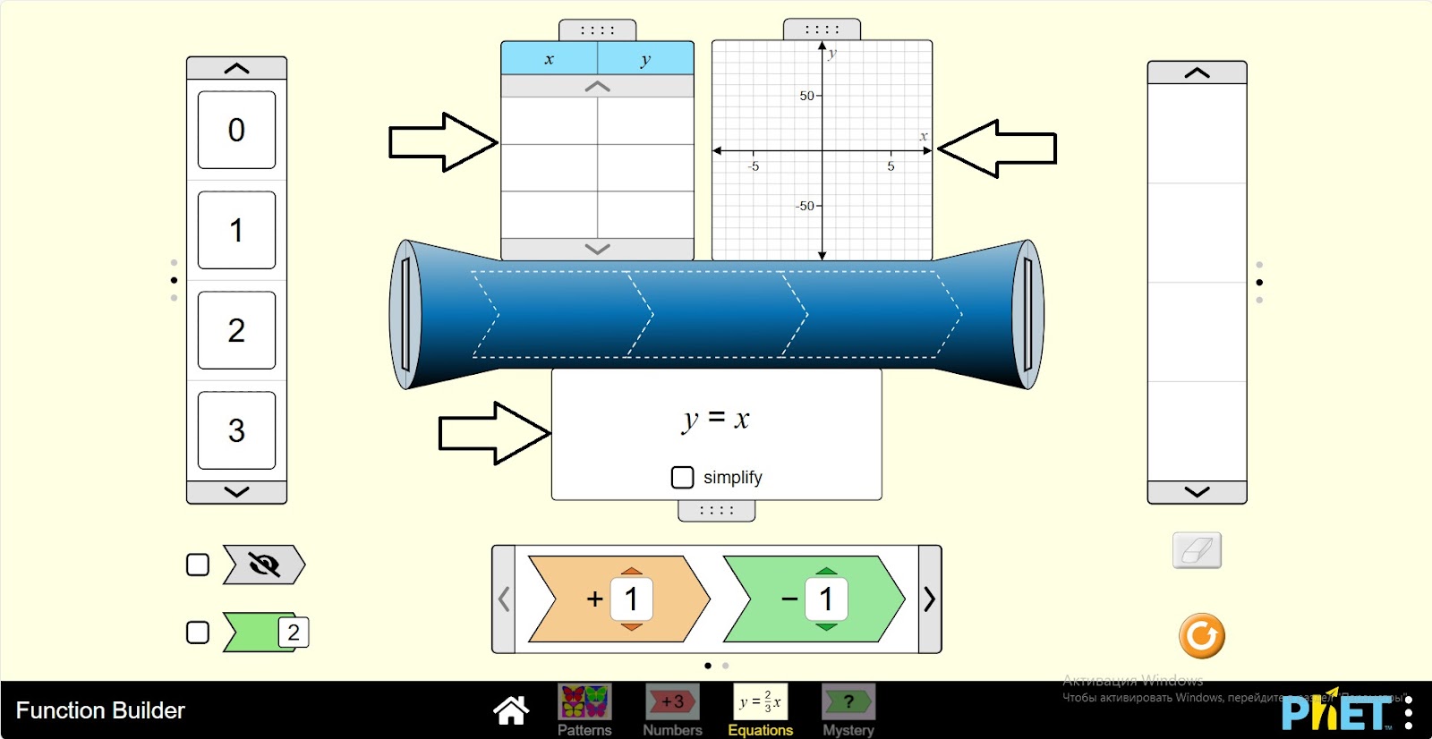
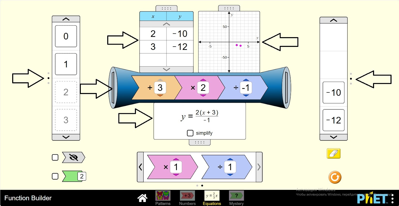
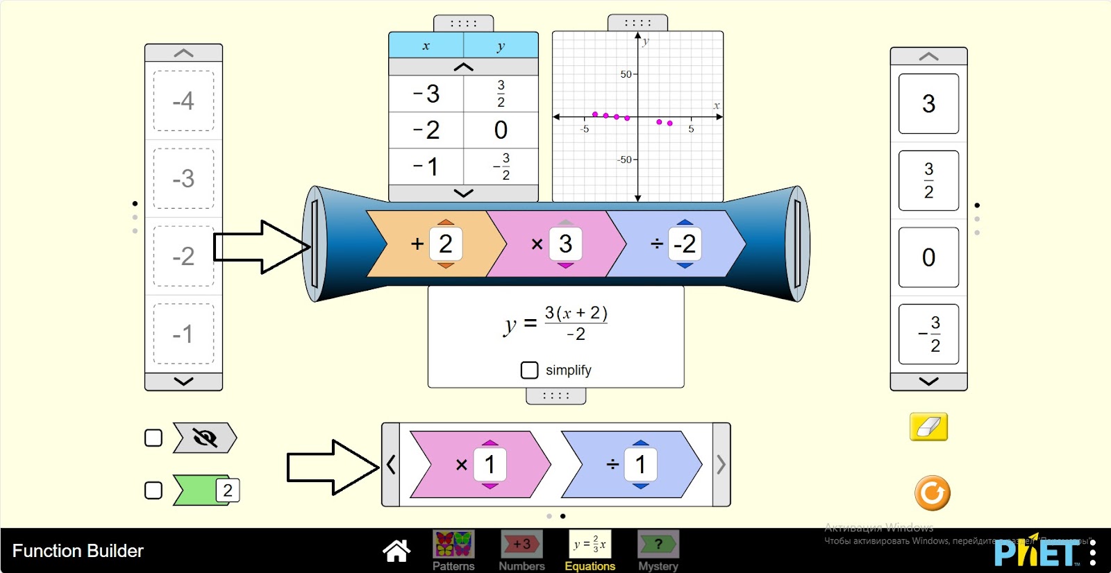
Step 4. Place an arithmetic operation on the function machine. You can change the numbers with an interval from -3 to +3. You can use addition, subtraction, multiplication and division operations.
Step 5. Enter the incoming number into the function machine. The input panel shows the numbers (-5; 7) and the variable x.
Step 6. You can see the number of inputs, function value, graph and equation in the tables. The function value panel shows the value of the expression.
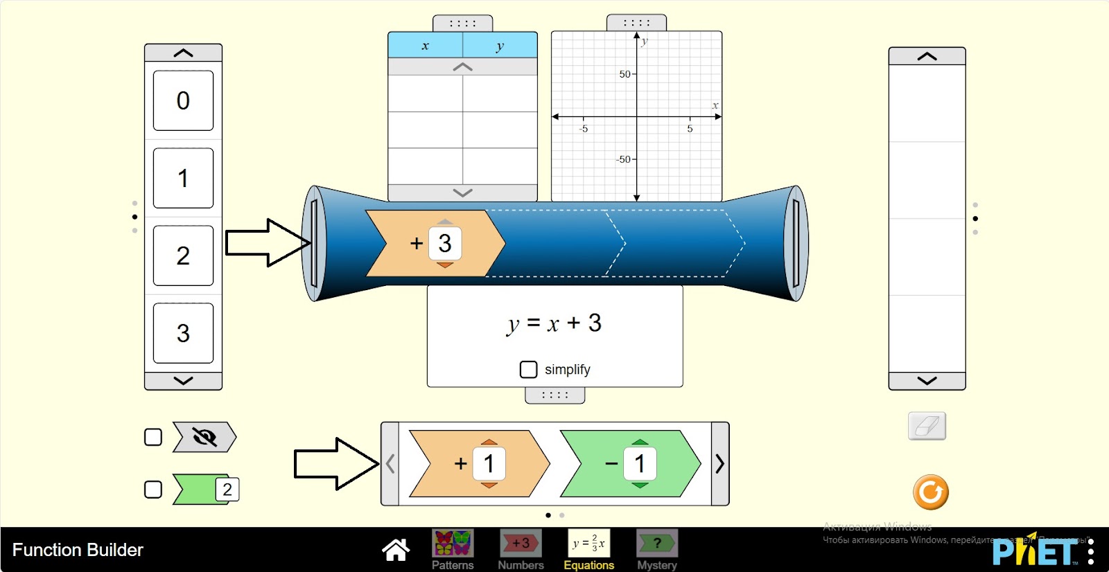
Step 7. Place more different arithmetic operations on the function machine. You can place up to three techniques there.
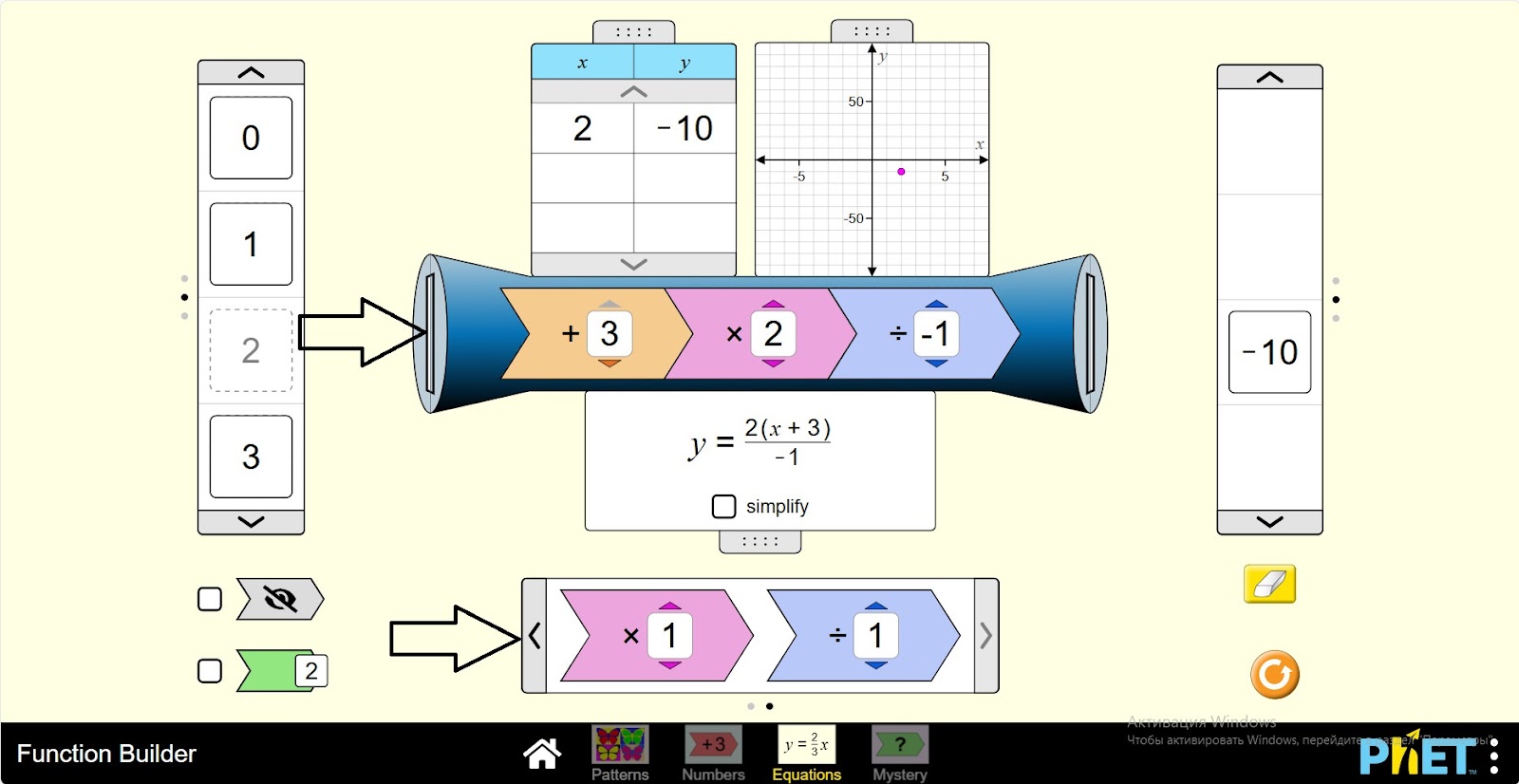
Step 8. Put the input number into the function machine. Examine the function data.
Step 9. Activate the button indicating the value of the expression. Enter the input number into the machine. After the first operation, the value of the expression is displayed.
Step 10. To perform the next operation, you pass the expression value to the next operation by holding down the left side of the mouse.
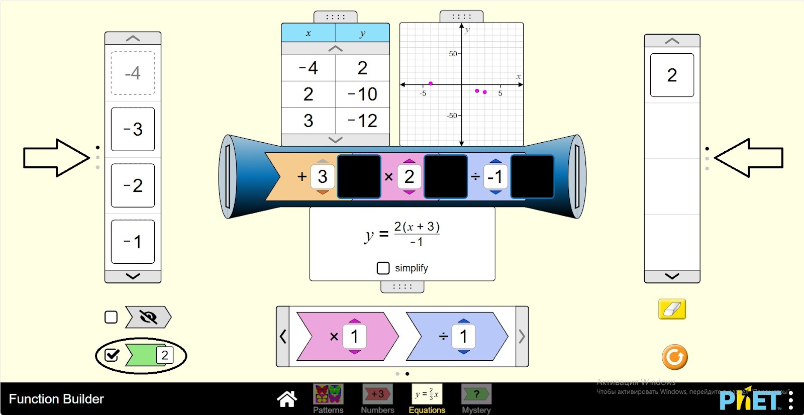
Step 11. Change the data as you see fit and create different expressions. You can use the input numbers panel, operations.
Conclusion
For students, working with a given function machine in virtual work is an easy way to explore functions and their effect on input data. Following the steps in sequence allowed them to experiment with different arithmetic operations and input numbers, and to observe changes in function values and equations.