
Vector: Equation of a line
Vector Addition: Equations by PhET Interactive Simulations, University of Colorado Boulder, licensed under CC-BY-4.0 (https://phet.colorado.edu)
Objective:
- To describe what happens when a vector is multiplied by a scalar;
- To graph vectors in order to add or subtract vectors;
- Learn and compare the results of each vector equation.
This virtual activity is designed for use in geometry lessons on the following topics:
- Grade 9. “Equation of a straight line”
Theoretical part
A vector is a directed line segment characterized by
- Beginning: The point from which the vector starts.
- End: The point to which the vector points.
- Length: The distance between the start and the end.
- Direction: Indicated by the arrow at the end of the vector.
Multiplying a vector by a scalar
Multiplying a vector by a scalar changes the length of the vector. If the scalar is positive, the direction of the vector is preserved; if it is negative, the direction is reversed.
Addition and Subtraction of Vectors
- Addition: Parallelogram rule or triangle rule.
- Subtraction: Subtracting a vector is the same as adding its opposite vector.
A line equation is a mathematical expression that defines all the points that lie on a given line in the plane. One of the most common ways to write the equation of a line is the general equation:
Ax + B + C = 0
where A, B, and C are some constant numbers, and at least one of A or B is not zero.
The geometric significance of the coefficients
- A and B: These coefficients determine the direction of the line.
- C: The coefficient C determines the position of the line with respect to the origin.
Virtual Experiment
In the “Vector Addition: Equations” virtual activity, students experiment with vector equations and compare vector sums and differences. Students learn about scalar multiplication by performing calculations with vectors and changing the coefficients in an equation.
Workflow:
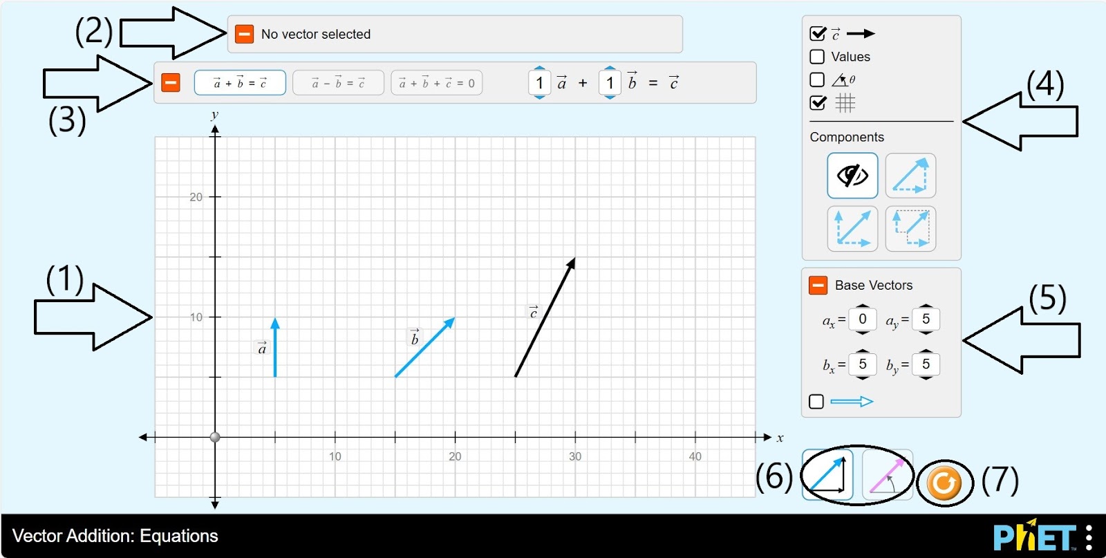
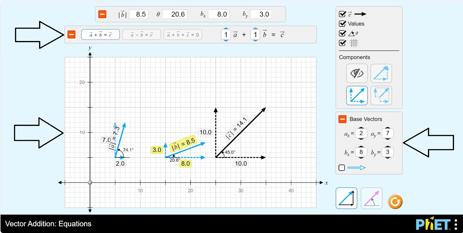
Step 1. Launch the simulation. In the workspace provided:
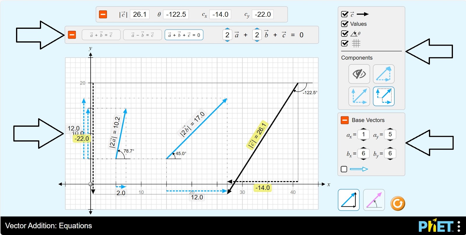
- The OXY coordinate plane containing the vectors a, b, c (1);
- A vector data table (2);
- The vector equation (3);
- c, dimension display, angle, grid, panel where component buttons are located (4);
- Vector coordinates panel (5);
- Vector type selection: by size, by angle (6);
- Reload button (7).
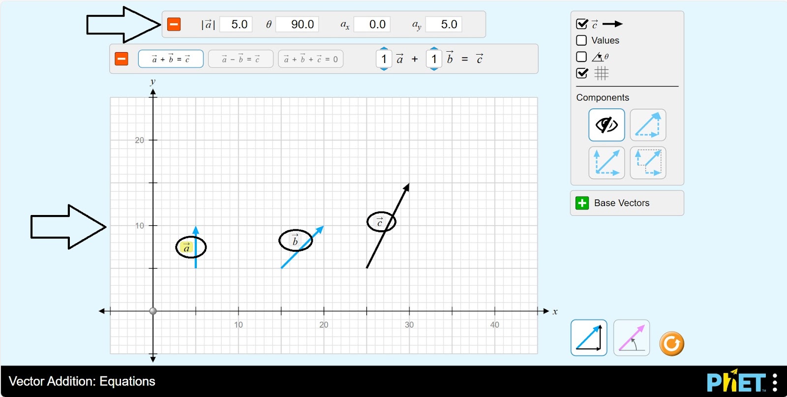
Step 2. Explore the information of the vector data panel by clicking vectors a, b, c.
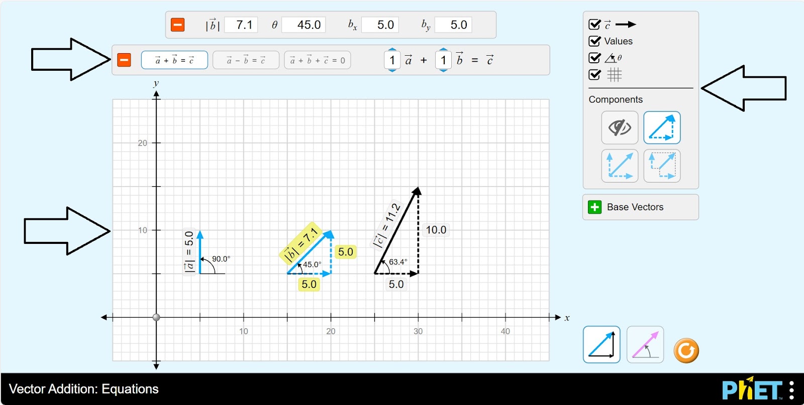
Step 3. Activate the “Values” and “Angle” buttons. Explore the different layouts of the vectors by clicking on each button in the Components panel.
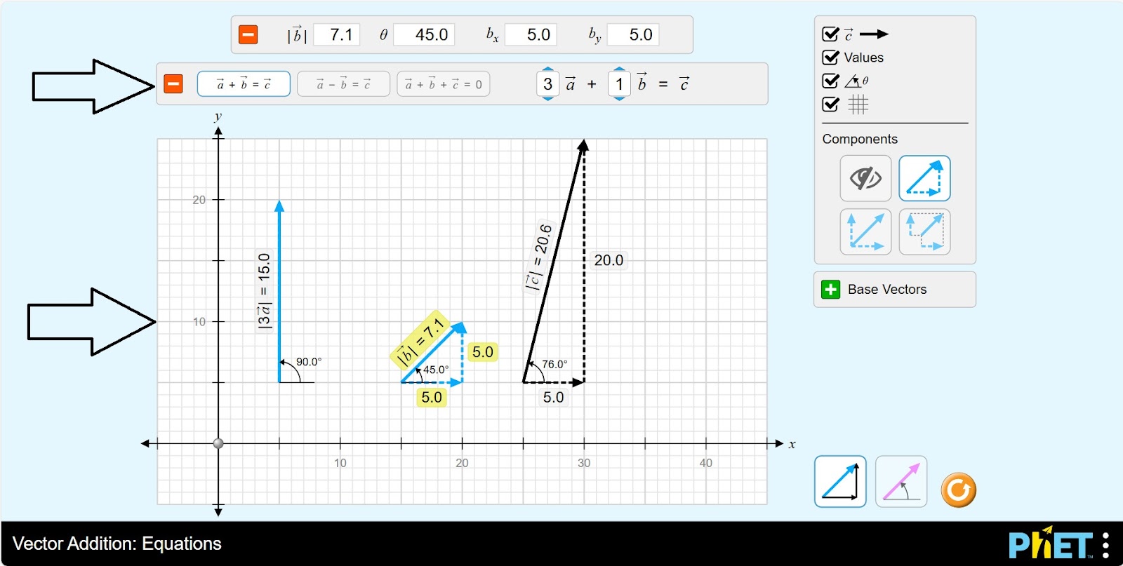
Step 4. Perform a vector calculation using the equation a+b=c. Change the coefficients of the vectors a and b and solve the problems.
Step 5. Modify the vectors a and b by changing the values ax, ay for the vector a, bx, by for the vector b from the vector coordinates panel. Since a+b=c, the vector c is changed automatically.
Step 6. Click the Reload button. Select the equation a-b=c.
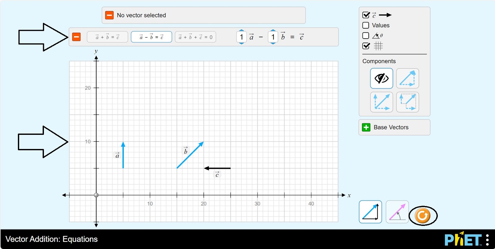
Step 7. Repeat the operations created for the equation a+b=c and examine the vectors.
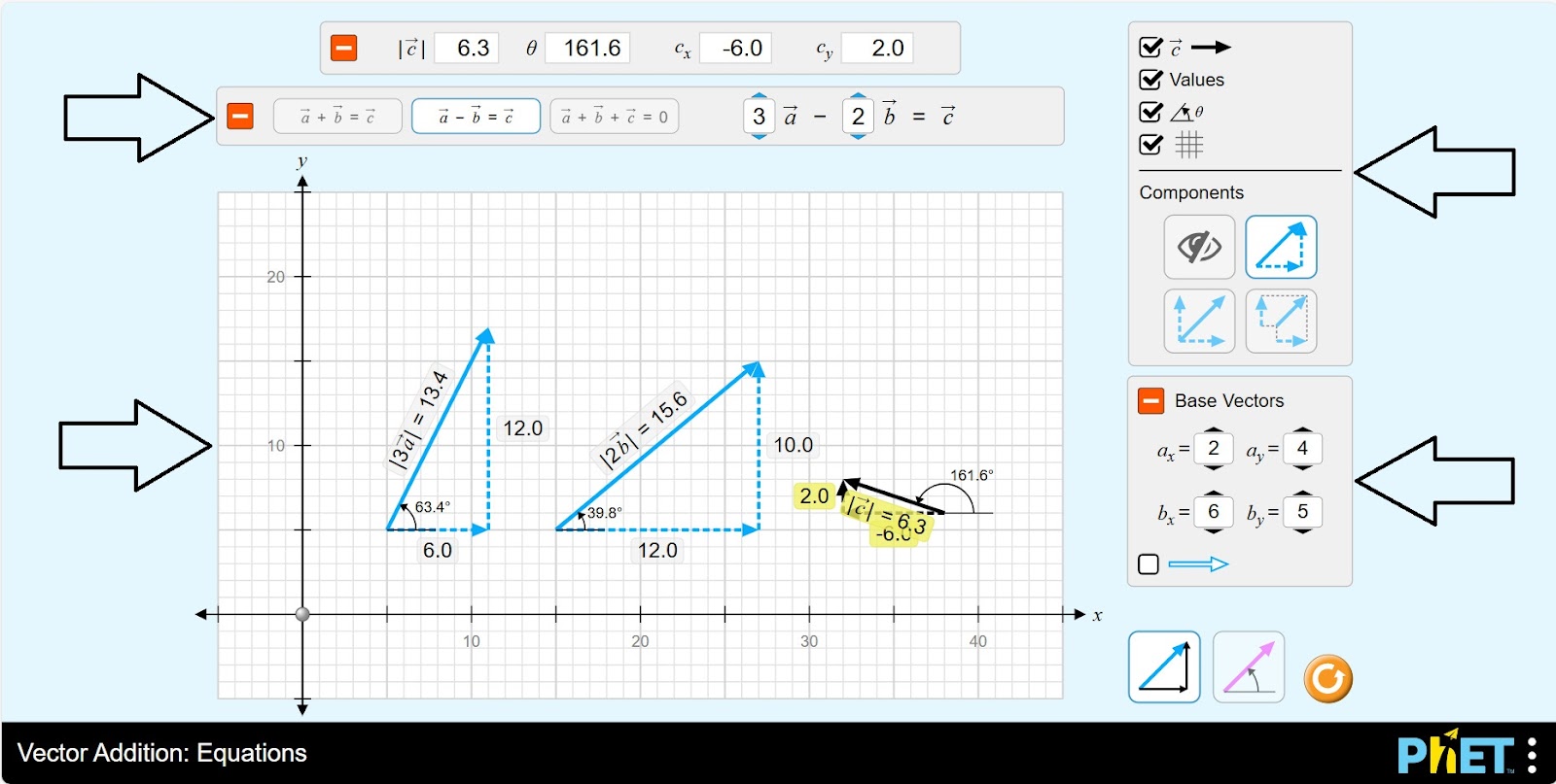
Step 8. Click the Reload button. Select the equation a+b+c=0.
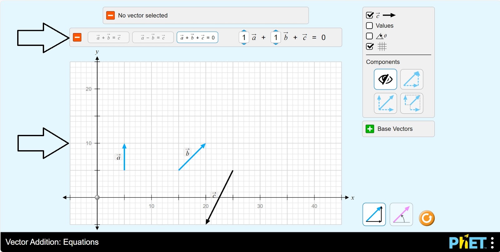
Step 9. Repeat the operations created for the equation a+b=c and examine the vectors.
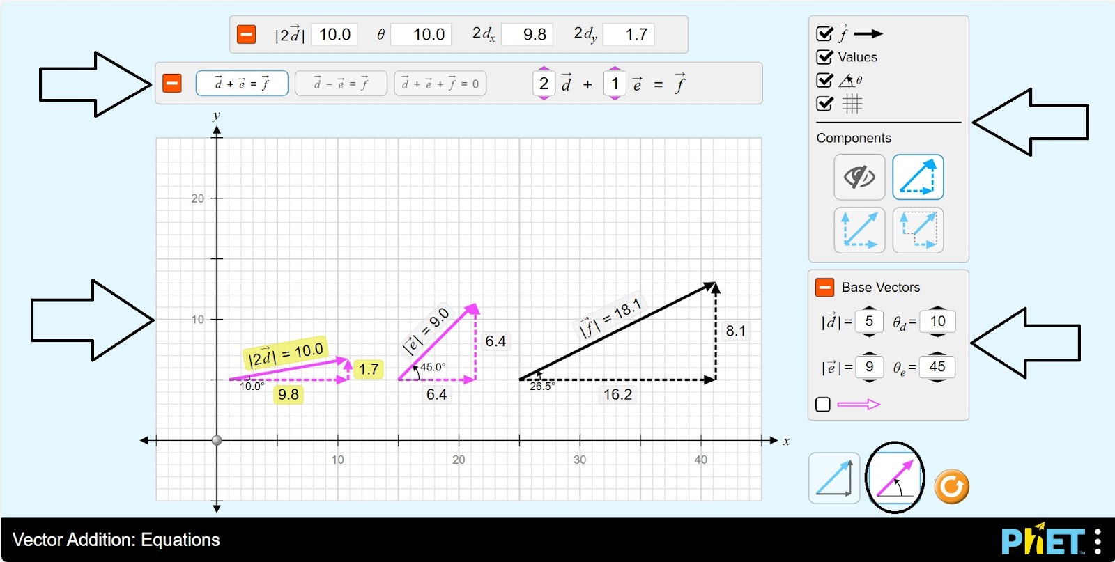
Step 10. You can select the vector type by angle and perform calculations for the vectors d, e, f.
Conclusion
Students learned more about the concept of a vector by working on this simulation. They studied and compared the changes that occur when a vector is multiplied by a scalar, and the results of adding and subtracting vectors. Mastered techniques for adding vectors using the parallelogram rule and the triangle rule.