
Lesson 1
Background
The influenza (flu) virus is responsible for many deaths in the world. It is most dangerous in the elderly, young children, and people with impaired immune systems. The flu virus is difficult to contain because it can be transmitted fairly easily through the air and skin contact. It also mutates quickly, and each year new strains arise. Each year, scientists must predict which strains are most likely to be responsible for flu outbreaks and produce vaccines specific to those strains. This is why people must be vaccinated for the flu every flu season – the previous year’s vaccine does not protect from new flu strains.
There are two types of flu vaccine. One has intranasal administration, and the other is injected. Pharmaceutical companies that produce these vaccines must decide each year when to start producing the vaccines, and also how much of each type of vaccine to make, given certain constraints on their budget, storage capacity, and so on. The longer they wait to begin production, the more accurate scientists’ predictions are likely to be.
Introduction
Introduce the situation to the class and tell students that they will be the production leaders at the pharmaceutical plant, which will produce some of each type of this year’s flu vaccine. Collect ideas about the considerations that must be taken into account when making a production decision like this one, and whether some of these considerations can be quantified. Introduce the concept of mathematical constraints as it pertains to this situation.
Pass out the How Much of Each Vaccine? worksheet. After giving students a chance to read it, ask the class to identify which of the five informational statements represents a constraint. They should notice that the first four statements reduce the production choices available to the plant, and are thus constraints. The fifth statement provides information that concerns the amount of time it takes to produce the vaccine, which is what needs to be optimized. Tell students that this will become part of the final solution once all of the constraints are taken care of.
Click to download the worksheet

Translating Inequalities Into Algebraic Statements
Have students translate the four constraints into algebraic inequalities and circulate among the class to see if it is necessary to review concepts of inequality. Students may need to be reminded that these inequalities should be more than or equal to (≥) and less than or equal to (≤). (The situation was intentionally written that way so that the corresponding graphical representation would have solid lines instead of dotted ones, which makes finding the solution much more straightforward.) Tell students that even though it is not stated because it is so obvious, the plant cannot produce negative amounts of intranasal or injected vaccines, and these are also constraints. Students can then record these equations for Question #2 on the worksheet.
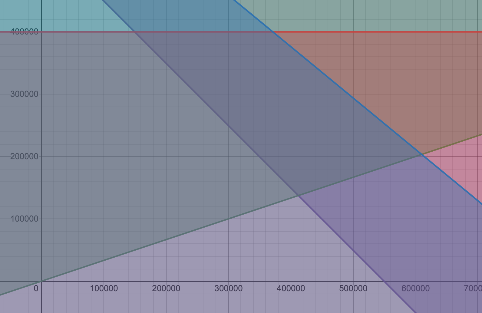
For convenience, the four inequalities are
N + I ≥ 550,000
3N ≥ I
N ≤ 400,000
$1.70N + $1.40I ≤ $1,200,000
Where N represents the number of intranasal vaccines produced, and I represents the number of injected vaccines produced.
Have students volunteer other phrases that translate into more than, less than, more than or equal to, and less than or equal to. This is the time for Algebra I students to have more practice translating inequalities before moving on to the next phase of this lesson.
Graphing Two-Variable Inequalities
Remind students that graphs are a visual way to display all of the solutions to a particular equation or inequality. For example, a first-degree, two-variable equation will produce a linear graph because there are infinite solutions that all happen to map to a straight line on the coordinate plane. Any coordinate that does not fall on that line is not a valid solution.
With that in mind, what would the graph of a two-variable inequality look like? You may choose to split the class into groups and have each group graph one constraint on an overhead transparency to share with the rest of the class. Agree on a scale for each axis that the entire class will use before assigning groups a constraint, and give each group a different colored pen to create their graph.
Students will discover that instead of a line, they produce a shaded half-plane. The plane is cut by a boundary line that was created by the constraint they were assigned. Emphasize that any point in the shaded region satisfies the constraint, and any point outside the region does not. Further, points on the boundary line itself also satisfy the constraint because of the way the inequality was written, which is why it is represented with a solid line instead of a dotted one.
Describing the Feasible Region
If the class produced their graphs on overhead transparencies, project the graphs for the class and check for any errors. Then lie all of the graphs on top of each other to see where the regions overlap. Ask students to explain the significance of this overlapping region. Students should state that this region defines the set of all possible decisions that would satisfy every constraint at the same time. Introduce the term feasible region.
Have groups create their own copies of the feasible region on graph paper.
Teachers of Algebra I classes may choose to end the lesson here. Alternatively, teachers of Algebra I classes may choose to skip the optimization part of the lesson and show students how to solve systems of equations to better define the boundaries of the feasible region.
Students might assume that if the feasible region were bounded by exclusive inequalities instead of inclusive ones, the best solution would be the point closest to the corner that would have been the optimal answer if it were part of the feasible region. This is not always the case, however, and finding solutions in situations like those require doing more difficult mathematical calculations.
Optimization
Now that the class has created a feasible region, which choice in that region would take the least amount of time to produce? This is where the last informational statement (#5) in the worksheet is used. Ask students to write an expression describing the amount of production time needed for a certain combination of intranasal and injected vaccine. The expression is
43N + 50I = Production Time
Any production choice in the feasible region will satisfy all of the constraints, but only one choice (in this case) will satisfy all of the constraints in the least amount of production time. The class could take the time to plug every possible production combination into the Production Time formula above to find the best solution, but of course there is an easier and faster method.
It is useful to understand the behavior of the production time function as the time allowed is increased. Ask students to graph the equation that gives the production choices available if the plant has only 100 hours to make flu vaccine. Then increase the allowed time to 500 hours, then 750 hours, then 1000 hours, etc. As the time allowed increases, ask the class to observe what happens to the graphed line. Students should notice that the slope of the lines that they are graphing remains the same, but the line itself shifts “outward” to correspond with the increased production capacity that more time allows. In other words, as you change the equation to increase the amount of time allowed, parallel lines are produced that move progressively farther away from the origin.
This situation calls for finding the least amount of production time possible, so students should realize that they would like their production time equation to be as close to the origin as possible while still including at least one point in the feasible region. Have students try to decide which is the best production decision. It might be helpful to use a ruler or piece of spaghetti to represent the optimization equation that can be shifted in or out. Students can shift the straightedge towards the origin until it hits the last possible point on the feasible region, the lower corner.
Solving Systems of Equations
The class has now conceptually found the solution to the problem, but must now calculate the exact answer. What are the coordinates of the optimal solution? If your class skipped the conversation about optimization, it is still helpful to know the corners of the feasible region in order to have a precise description of its shape. Hopefully the class chose a scale for the x- and y- axes that does not make the coordinates of the corners obvious. Show the class that the corners of the feasible region are simply intersections of two constraints, and thus can be found by solving a system of two simultaneous equations. Provide instructions on solving systems of equations algebraically, allowing groups to solve for each of the four corners of the feasible region.
For convenience, the corners of the feasible region are (150,000, 400,000), (371,439, 400,000), (600,000, 200,000), and (412,500, 137,500). The optimal solution is to produce 412,500 injected vaccines, and 137,500 intranasal vaccines.
Discussion
Ask the class to agree on the best production decision for the pharmaceu- tical plant. Tell students that such major decisions are to be documented for later reference, and have them produce a brief justification of their final decision by summarizing the logic of their decision-making process.
Talk about other contexts in which linear programming would be useful.
Extension/variation
Invite a flu vaccine specialist to be a guest speaker, perhaps in Science class, about how the flu vaccine is chosen each year.