
A linear function and its graph
Graphing Slope-Intercept by PhET Interactive Simulations, University of Colorado Boulder, licensed under CC-BY-4.0 (https://phet.colorado.edu)
Objective:
- To know the definition of the function y=kx, construct its graph and establish its location as a function of k;
- Know the definition of the linear function y=kx+b, construct its graph and determine its location depending on the values of k and b;
- Finding the points of intersection of the graph of a linear function with the coordinate axes (without graphing);
- Determining the signs of k and b of the linear function y=kx+b given a graph.
This virtual work is intended for use in algebra lessons on the following topics:
- Grade 7. “Linear function and its graph”
Theoretical part
Definition of linear function
A linear function is a function that can be written in the form:
- y = kx, where k is the coefficient of proportionality, or
- y = kx + b, where k is the angular coefficient, b is the free term.
The graph of a linear function is always a straight line.
Graph of the function y = kx
The coefficient k determines the slope of the straight line:
- When k > 0, the straight line is increasing (pointing upward from right to left).
- When k < 0, the line is decreasing (pointing downward from right to left).
- At k = 0, the straight line is parallel to the Ox axis (is the Ox axis).
The graph of the function y = kx always passes through the origin (point (0; 0)).
Graph of the function y = kx + b
- The free term b determines the point of intersection of the graph with the Oy axis.
- The angular coefficient k determines the slope of the line, as in the case of the function y = kx.
- The graph of the function y = kx + b is parallel to the graph of the function y = kx and is shifted along the Oy axis by b units upward if b > 0, and by |b| units downward if b < 0.
Finding points of intersection of the graph with the coordinate axes
The point of intersection with the Oy axis:
Substitute x = 0 into the equation of the function and find the value of y. Coordinates of the intersection point: (0; b).
Point of intersection with the Ox axis:
Substitute y = 0 into the equation of the function and solve the equation kx + b = 0 with respect to x. Coordinates of the intersection point: (-b/k; 0).
Determining the coefficients k and b from the graph
Coefficient b:
We find the point of intersection of the graph with the Oy axis. Its ordinate is the value of b.
Coefficient k:
Choose any two points A(x1; y1) and B(x2; y2) on the graph.
We use the formula: k = (y2 – y1) / (x2 – x1).
Virtual experiment
In the Graphing Slope-Intercept simulation, students explore a line at an angle of slope. Draws a sloping line through the equation of a given graph. Predicts how changing the values in the linear equation will affect the line shown on the graph. Predicts how changing the line shown on the graph will affect the equation.
Course of Work:
Section 1. Slope-Intercept Part
Step 1. You will be given 2 different modes, “Slope-Intercept” and “Line game”. Start the “Slope-Intercept” mode.
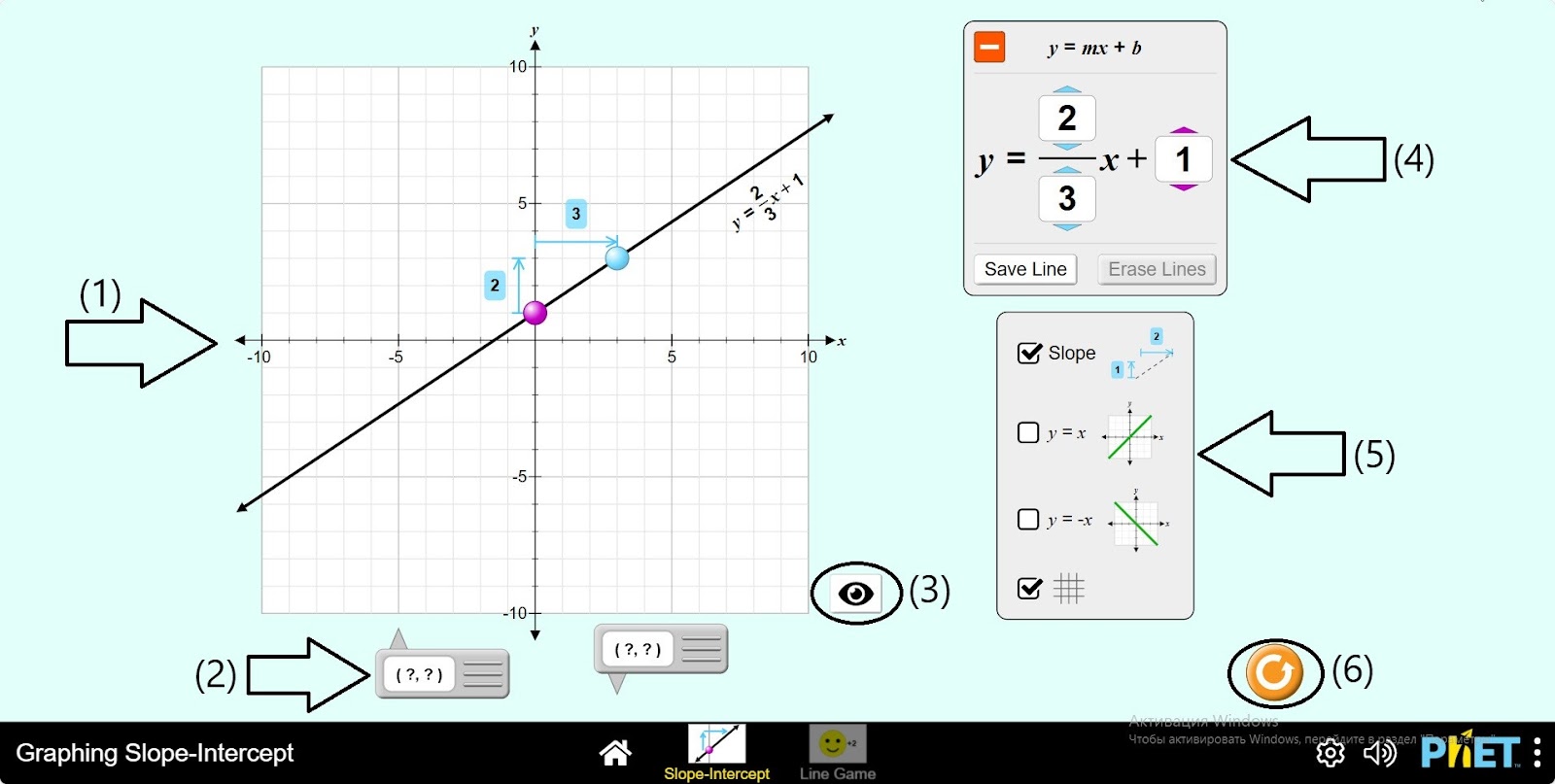
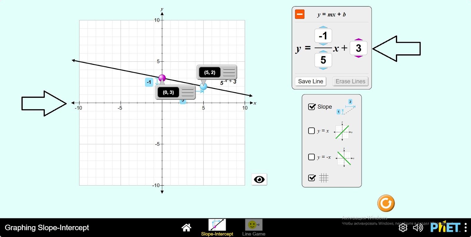
Step 2. You are given:
- The OXY coordinate plane and a graph of y = ⅔x + 1 (1);
- Tools that show the values of the points (x,y) in the graph coordinate (2);
- You can keep the graph off the screen by clicking on the eye (3);
- Equation y = mx + b, buttons that change the values of m, b (4);
- Buttons to save and turn off the graph type (5);
- Buttons show slope, show graphs of y = x and y = – x (6);
- Reload button (7).
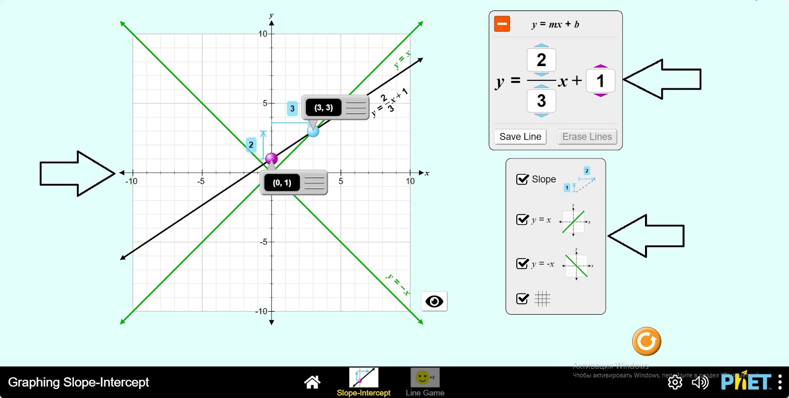
Step 3. Determine the points of the graph of y = ⅔x + 1 using the tools that show the values of the points (x, y) in the graph coordinate. add buttons to show graphs of y = x and y = – x. Examine the graph.
Step 4. Change the values of m, b of the function y = mx + b and study the graph.
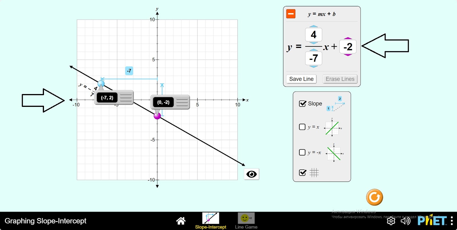
Step 5. Examine the graph by changing the m, b values of the function y = mx + b. You can use the buttons and tools provided on the screen. Make some calculations.
Section 2. Game Part
Step 6. Activate the “Line Game” mode. You are given 4 levels. Select the first level.

Step 7. You are given:
- Graph Equation Plate (1);
- The OXY coordinate plane and the graph of y = mx + b (2);
- Tools showing the values of the points (x,y) in the graph coordinate (3);
- Check button (4);
- Back to menu button (5).
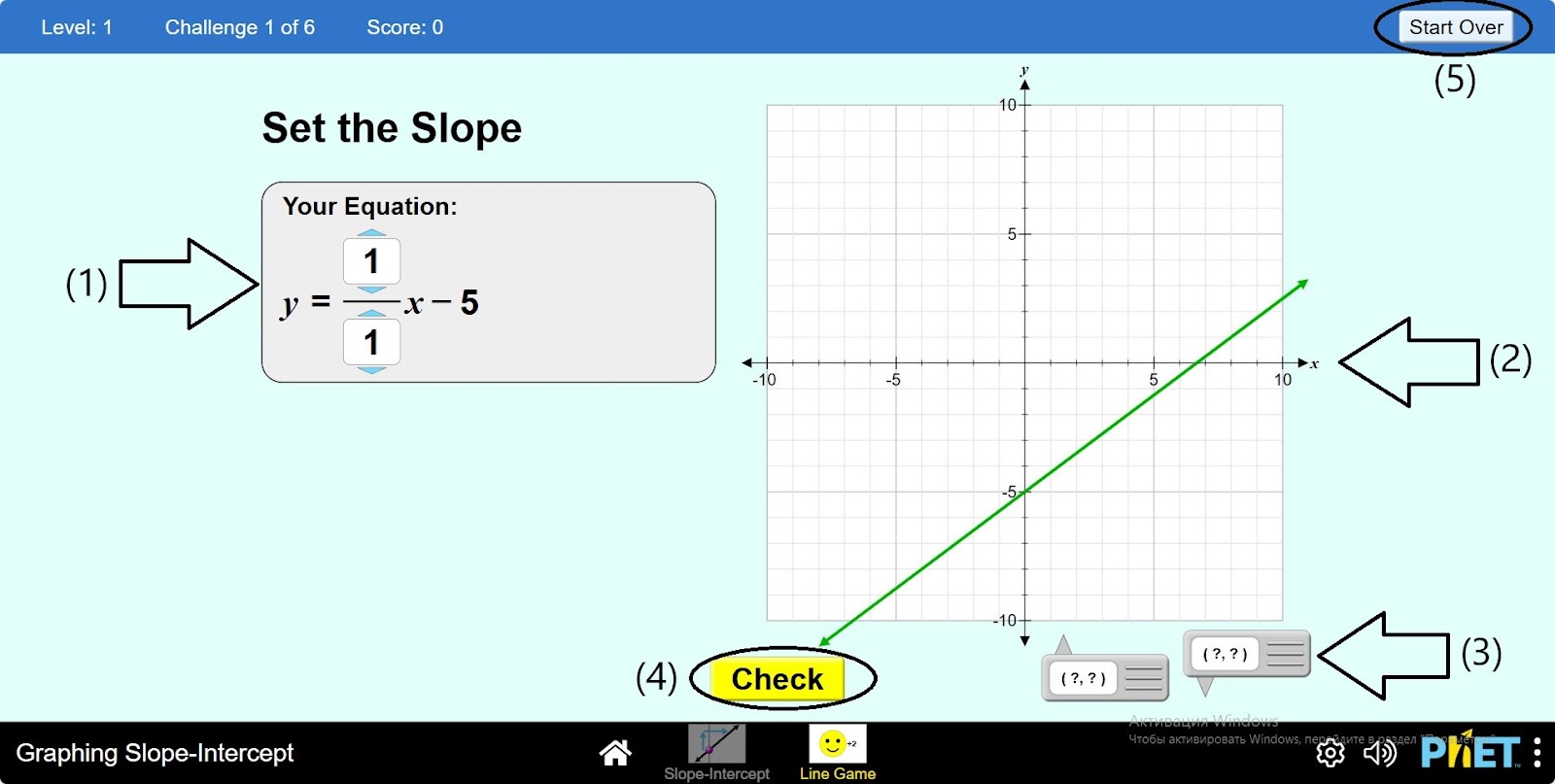
Step 8. You have an equation or graph in green. This is the task you must complete:
- If the graph is green, you must create an equation that fits the graph correctly;
- If the equation is green, you must create a graph that fits the equation correctly.
Complete and review the assigned problem.
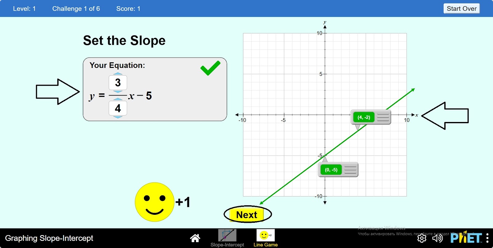
Step 9. Complete the assignment and move on to the next level.

Conclusion
The virtual lab is a valuable tool for students to learn the graphs of linear functions. The simulator has become interactive and visually useful by providing various tools for learning graphs, such as displaying points, displaying equations, and saving graphs.