Linear Function: Slope of Graph

<br />

Graphing Lines by PhET Interactive Simulations, University of Colorado Boulder, licensed under CC-BY-4.0 (https://phet.colorado.edu)

Objective:

To know the definition of the function y=kx, to construct its graph and to find its location according to k;
Know the definition of the linear function y=kx+b, construct its graph, and find its location given the values of k and b;
Find the points of intersection of the graph of a linear function with the coordinate axes (without constructing the graph);
Determine the signs of k and b of the linear function y=kx+b given by the graph.

This virtual work is intended for use in algebra lessons on the following topics

Grade 7. “Linear function and its graph”

Theoretical part

The slope of a graph, or angle coefficient, shows how steeply the line rises or falls. It is a key parameter for describing linear functions and has many practical applications.

Formula for Calculating the Slope

The following formula is used to calculate the slope of a line passing through two points (x₁, y₁) and (x₂, y₂):

m = (y₂ – y₁) / (x₂ – x₁), where:

m – slope of the line
x₁ and y₁ – coordinates of the first point
x₂ and y₂ – coordinates of the second point

What the slope means:

m > 0: The line ascends from left to right.
m < 0: The line slopes from left to right.
m = 0: The line is horizontal.
m is undefined: The line is vertical (x₁ = x₂).

How to use the formula:

Select two points on a line whose coordinates are known.
Substitute the coordinate values in the formula.
Perform the calculations. The resulting number is the slope of the line.

Virtual Experiment

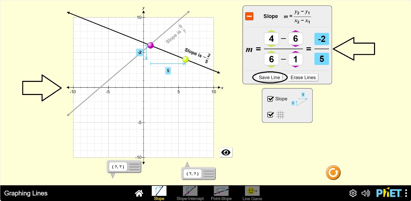
In the Slope Screen simulation, students explore the parameters of the slope formula and how changing the graph affects the equation or how changing the equation affects the graph.

Course of Work:

Part 1. “Slope”

Step 1. You are given 4 different modes, “Slope”, “Slope-Intercept”, “Point-Slope”, and “Line game”. You will work in the “Slope” and “Line Game” sections. Start the “Slope” mode.

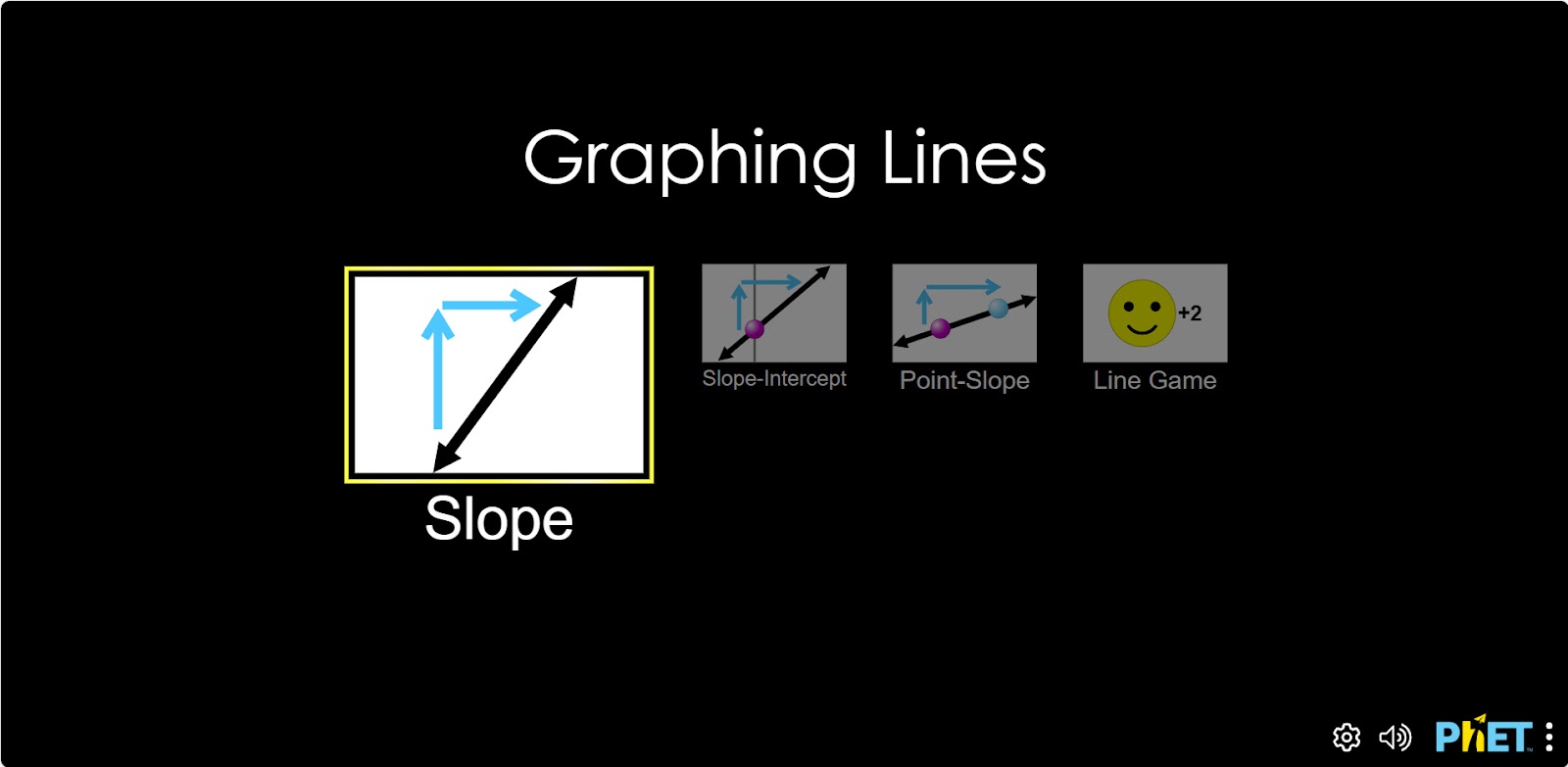
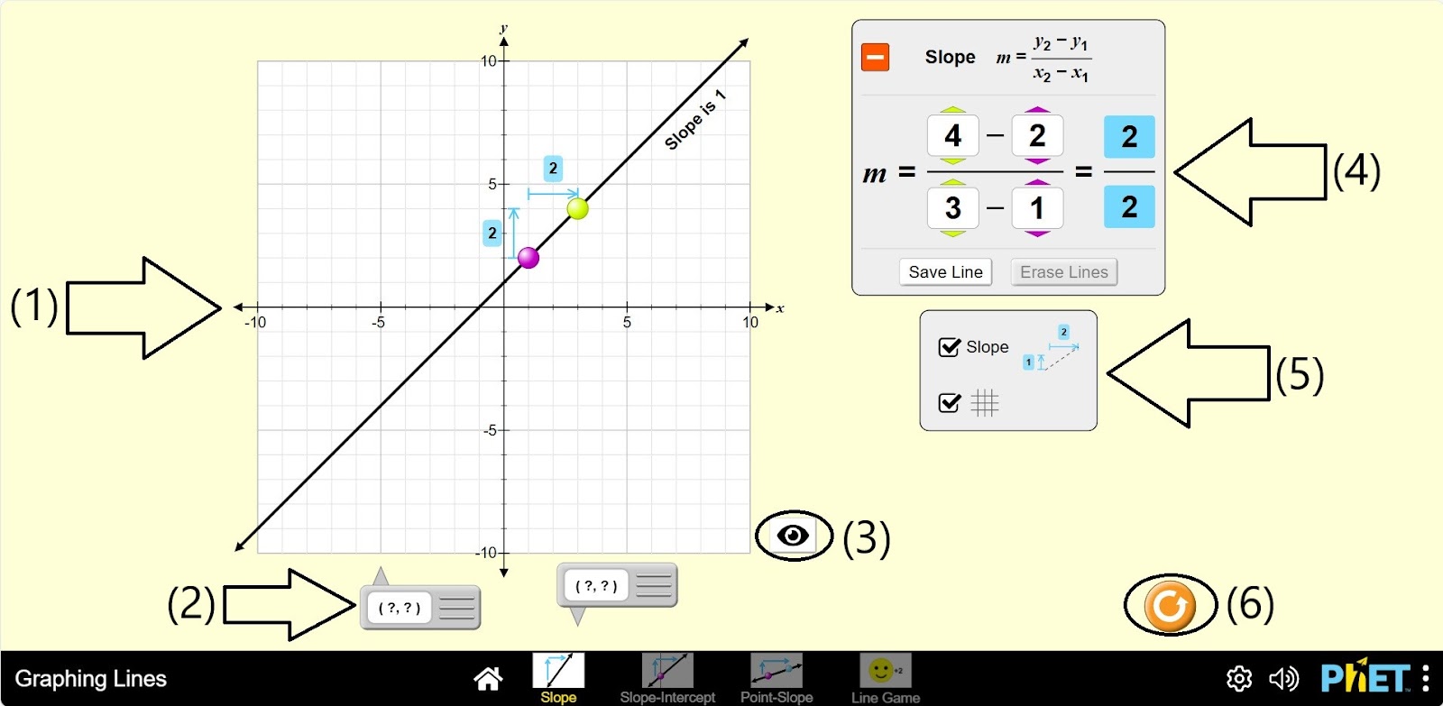
Step 2. You are given:

An OXY coordinate plane and a graph (1);
Tools that show the values of the points (x,y) in the graph coordinates (2);
You can keep the graph off the screen by pressing the eye button (3);
Slope equation: m = (y₂ – y₁) / (x₂ – x₁), and buttons to change the values of (x₁, y₁) and (x₂, y₂) (4);
Buttons for saving and turning off the graph type (5);
Slope parameter display, grid display buttons (6);
Reload button (7).

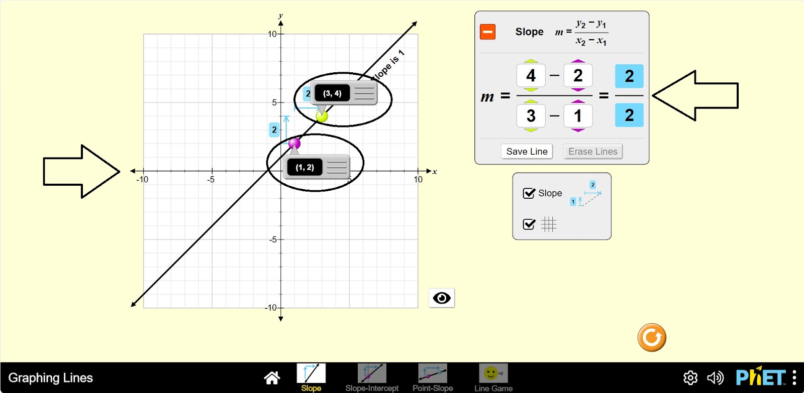
Step 3. Determine the points on the graph using the tools that display the point values (x, y) in graph coordinates. Examine the slope equation.

Step 4. Change the values of (x₁, y₁) and (x₂, y₂) from the slope equation. Examine the graph.

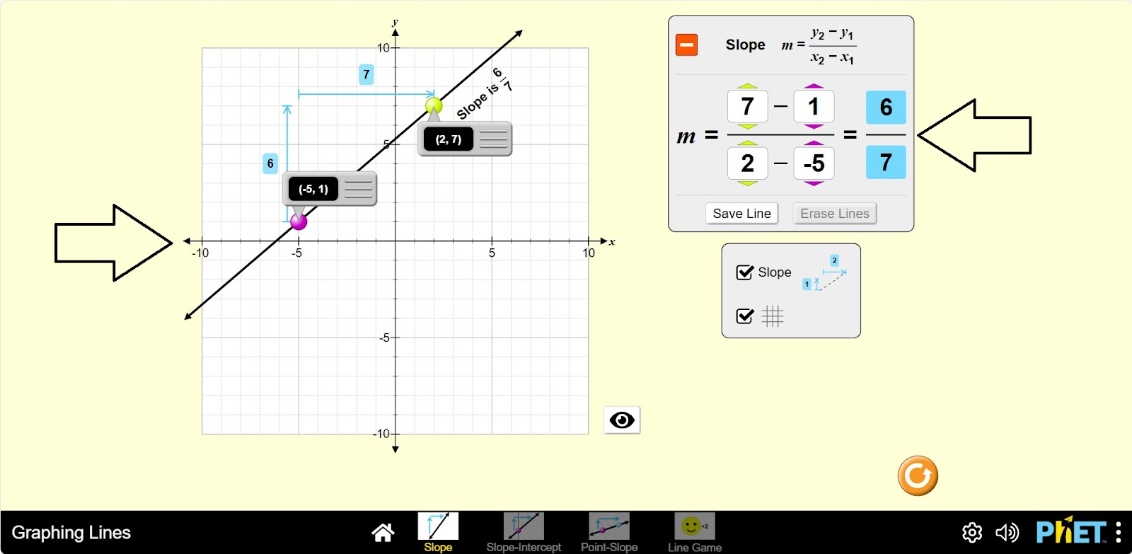
Step 5. Save the graph type, make some more graphs, and make comparisons with the slope equations.

Part 2. The Game Part

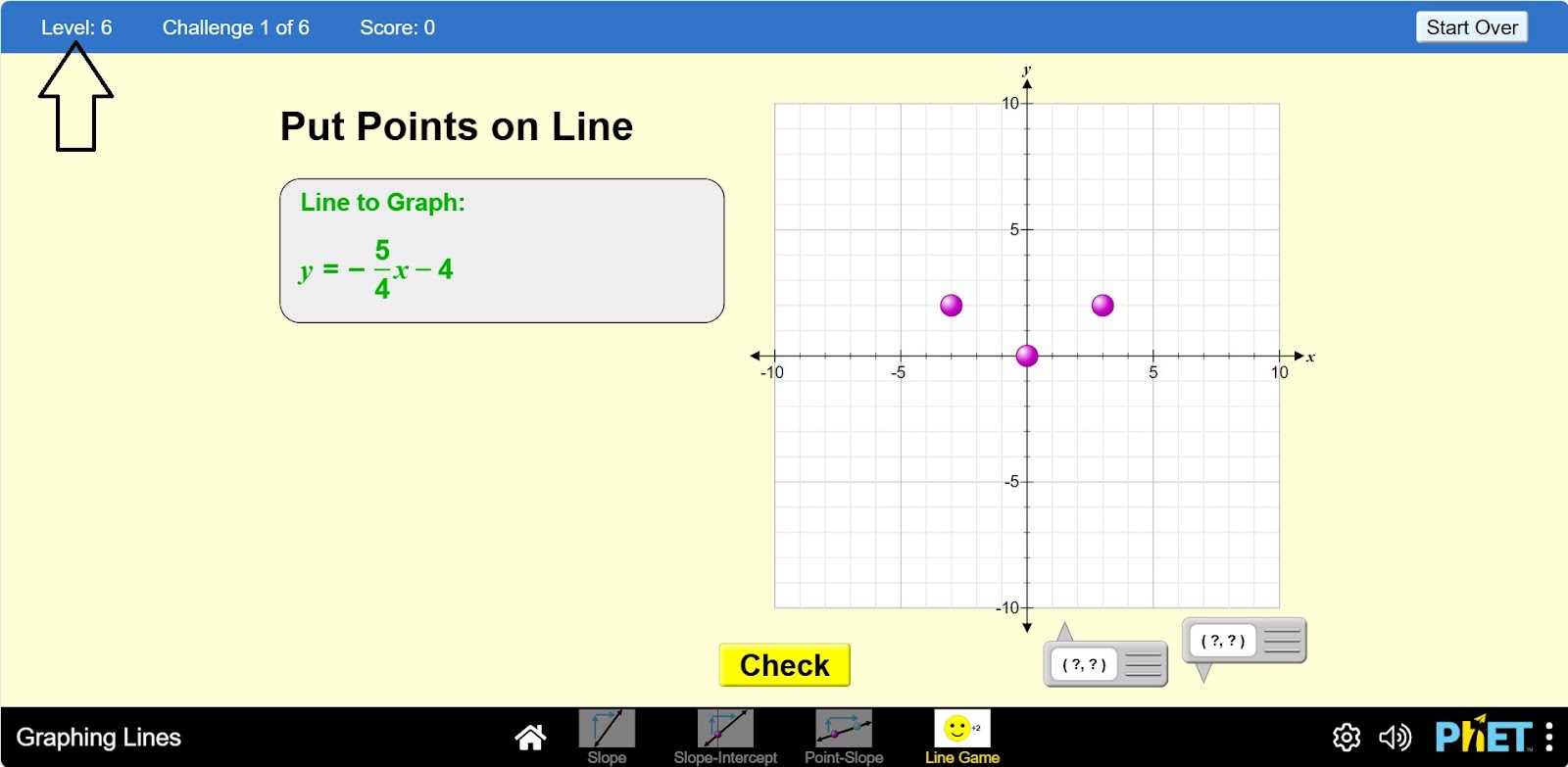
Step 6. Activate the “Line Game” mode. You will be given six levels. In this activity, you will work on levels five and six. Select the fifth level.

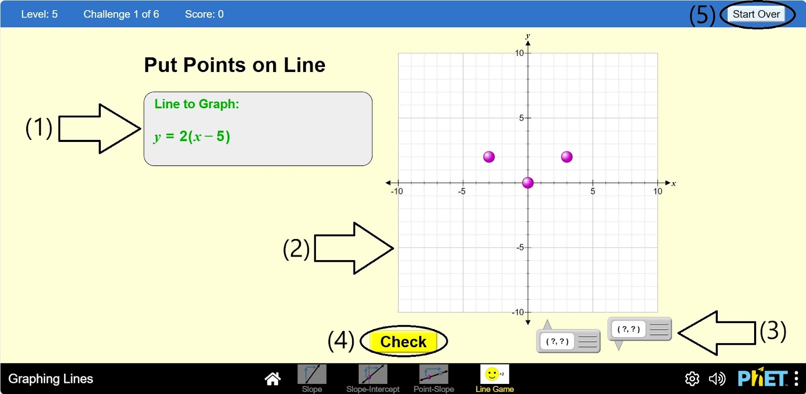
Step 7. You are given

Graph Equation Plate (1);
An OXY coordinate plane and a line graph (2);
Tools that display the values of the points (x,y) in the graph coordinate (3);
Check button (4);
Back to menu button (5).

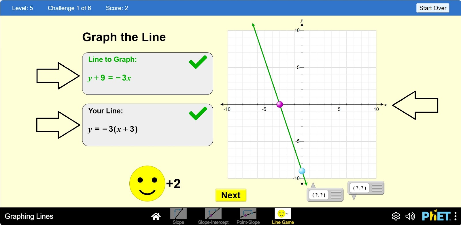
Step 8. You have an equation or graph in green. This is the task you must complete:

If the graph is green, you must create an equation that fits the graph correctly;
If the equation is green, you must create a graph that fits the equation correctly.

Complete and review the assigned problem.

Step 9. Complete the assignment and move on to the next level.

Conclusion

This virtual work is a slope formula for linear functions for students and a valuable tool for learning graphs. The simulator has become interactive and visually useful by providing various tools for learning graphs, such as displaying points, displaying equations, and saving graphs.